Vesimulus - Help!
Topics
- Bacterial Photosynthesis
- Simulation technique: the stochastic pools-and-proteins-model
- Protein models and parameters used in the simulation
- References
Preface
The following documentation is a short compilation from references [1], [2], and [3]. Many technical details and the biological reasoning for implementing things the way as we did, which are omitted here, are explained there in detail. In these publications you also find the references to the published rate constants or how we estimated their values.To make you more familiar with vesiweb, check out the tutorials, which introduce you into how to use vesiweb and what you can do with it.
Bacterial Photosynthesis
Photosynthesis in general is the synthesis of organic molecules using energy from light. It can be divided into primary and secondary reaction. During the secondary reaction, the products of the primary reaction are used to synthesize energy storing molecules (mostly glucose). The processes in the chromatophore vesicles of Rhodobacter sphaeroides, which are modelled here, belong to the primary reaction.The processes
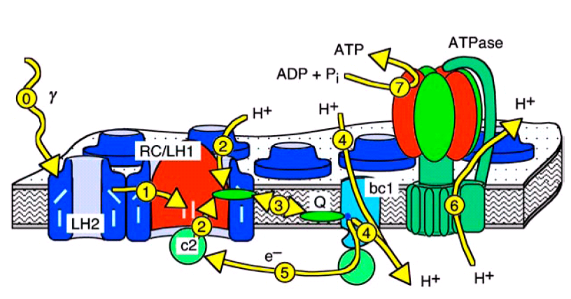 Figure 1: Textbook view of the photosynthetic
apparatus of Rb. sphaeroides.
Figure 1: Textbook view of the photosynthetic
apparatus of Rb. sphaeroides.
In purple bacteria light is absorbed by the light harvesting complexes of types 1 and 2 (LH1 and LH2, process 0 in figures 1 and 2), is then funneled to the reaction center (RC), and converted there into an electron proton pair (processes 1 and 2). Two of these pairs are then transported by one of the membrane bound quinone molecules to the cytochrome bc1 complex (bc1, process 3). There, the two protons are released to the interior of the vesicle, while the energy of the electrons is used to pump another two protons into the vesicle (process 4). The electrons are returned to the RC by the water soluble protein cytochrome c2 (c2, process 5), which is confined to the interior of the vesicle. The proton gradient across the vesicle membrane is finally used by the F0-F1-ATP synthase (ATPase) to synthesize ATP (processes 6 and 7).
The size of the vesicles
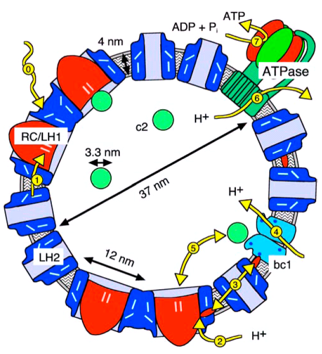 Figure 2: Cross section drawn to scale through a
chromatophore vesicle from Rb. sphaeroides with a typical outer
diameter of 45 nm diameter.
Figure 2: Cross section drawn to scale through a
chromatophore vesicle from Rb. sphaeroides with a typical outer
diameter of 45 nm diameter.
All relevant process take place inside of the vesicle, which allows for natural and well defined boundary conditions. Also, the vesicles are so small, that the transport processes are much faster than the relevant association and dissociation reactions.
Consequently, the numerical requirements to simulate a complete vesicle are such, that their dynamics can be simulated almost in realtime with a time step of 10 microseconds.
Simulation technique: the stochastic pools-and-proteins-model
The "Pools-and-Proteins" ain't a Pub..
Depending on your background you might have a different idea than figures above popping up in your mind, when someone says "photosynthesis!": you might think of a conversion chain from light into chemical energy or have a more mechanical picture. This view even made it onto the cover of the Biophysical Journal. None of these views on its own is completely correct or even completely wrong.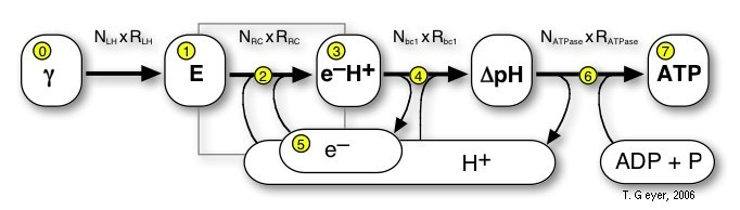
Here we use a "pools-and-proteins" model, which combines the details of individual proteins, each with their own set of discrete internal states and binding sites, and the network view of uniform concentrations of a discrete number of indistinguishable metabolite molecules. Thus, the proteins are the "machines" where the conversion between the metabolites takes place. Before this conversion can take place, the freely diffusing metabolite has to bind to a specific binding site on the protein. Then the protein acts on that bound metabolite and releases the respective product(s) again. Correspondingly, in our approach the proteins have a set of standard input and output connectors, by which the metabolites are taken up or put back into the pools. The model of a biological system therefore consists of the repsctive number of independent copies of each type of protein and one pool for each of the metabolites.
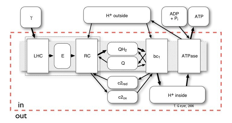
Figure 3: Schematic network like overview of the
relationships of all Proteins (rectangles) and Pools (rounded rectangles)
of the photosynthetic system of Rb. sphaeroides. The shaded gray
area indicates the membrane, which is not explicitly modelled, the red
broken line denotes, which pools are inside of the vesicle and which are
the external pools of the cytoplasm.
Binding and unbinding kinetics
In the model every reaction is modelled as the binding or unbinding of discrete molecules according to the respective rate constants kon or koff. However, a reaction can only take place conditionally, i.e., when the repsctive binding sites are empty (for an association reaction) or occupied with a product molecule (for dissociation). If the condition is fullfilled, a reaction probability P is determined. The reaction then takes place, when P is smaller than a random number from the range [0..1].For an association reaction
A + B -> AB
with its rate constant kon the rate of binding events of molecules B at a single protein A, Ron, is proportional to the density of B, [B]:
Ron = kon [B]
When the timestep is small enough, the probability Pon that one of the B molecules in a pool of volume V binds to A during a timestep ∆t is well approximated byPon = ∆t kon / V.
This Pon is then used in each timestep to statistically
let the reaction take place.
For an unbinding reaction
A:B -> A + B
a different strategy is used: here the rate of events is independent of the concentration of [B] and the probability needs not be determined anew in every timestep. Thus, form the dissociation rate constant koff a lifetime toff is chosen from an exponential probability distribution P(toff):P(toff) = exp[-toff koff]
With toff a timer is initialized, which then triggers the actual unbinding of B.Protein models, pools and parameters used in the simulation
Light Harvesting Complexes (LHC)
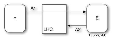 Figure 4: Model of the LHC with the included
reactions A1 and A2 and the associated photon and exciton pools (rounded
rectangles).
Figure 4: Model of the LHC with the included
reactions A1 and A2 and the associated photon and exciton pools (rounded
rectangles).
The LHC has no internal binding sites and contains two reactions, which model the photon capture (A1) and the eventual decay of unused photons (A2). The decay rate of excitons is modelled as
R(A2) = kd exp[N/N0]
- A1: kon = 2.44 m2/(s W)-1
- A2: kd = 103 s-1
- A2: N0 = 2
Reaction Center (RC)
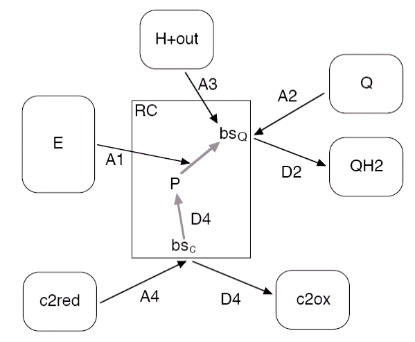 Figure 5: Reactions and binding sites of the
RC (rectangular box) and the connected pools (rounded boxes).
Figure 5: Reactions and binding sites of the
RC (rectangular box) and the connected pools (rounded boxes).
The binding reaction A2 (A4) can only take, if the binding site bsQ (bsc) is empty, whereas A1 and A3 depend on the oxidation state of P and Q
The intermediate steps from P to Q
The following table lists the reactions with their respective rate constants and their vesiweb labels. The rate for A1 is currently fixed.
| label | reaction | rate | vesiweb label |
| A1 | exciton-initiated electron transfer from P to Qb | 1010 s-1 | (n.a.) |
| A2 | quinone binding | 1.25 x 10⁵ nm2s-1 | Q kon |
| D2 | quinol unbinding | 40 s-1 | QH2 koff |
| A3 | proton uptake and transfer to Qb- | 1010 nm3s-1 | H+ outside kon |
| A4 | binding of reduced c2 | 1.4 x 10⁹ nm3s-1 | c2red kon |
| D4 | reduction of P and unbinding of oxidized c2 | 103 s-1 | c2ox koff |
The number of RCs is derived from the number of LHCs: A monomeric LHC has one RC, that accesses its private excitation pool, while a dimeric LHC feeds into two RC via a single exciton pool.
Cytochrome bc1 complex (bc1)
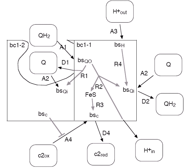
Figure 6:
Overview of the reaction of the modelled bc1 dimer. Of
the left half of the dimer, labelled bc1-2, only those parts are shown that
are relevant for the function of the other half. Note that the figure does
not reflect the respective stoichiometries of the reactions nor that the rate
of the internal reaction R2 is reduced with increasing transmembrane potential.
The rate of the central internal reaction of the bc1, in which the protons are pumped against the transmembrane potential ∆Φ, is modelled as
k2(∆Φ) = k2 exp[-∆Φ/∆Φ0]
| label | reaction | rate | vesiweb label |
| A1 | QH2 binding at Qo | 1.5 x 10⁵ nm2s-1 | QH2 kon @ Qo |
| D1 | Q unbinding from Qo, if Q was not transferred directly to Qi of the other half in reaction R1 | 180 s-1 | Q koff @ Qo |
| A2 | Q binding at Qi | 1.5 x 10⁵ nm2s-1 | Q kon @ Qi |
| D2 | QH2 unbinding from Qi | 180 s-1 | QH2 koff @ Qi |
| A3 | binding of a proton from the outside | 1010 nm3s-1 | H+ outside kon |
| A4 | binding of oxidized c2 with a mutual inhibition of the two binding sites of the dimer | 1.4 x 10⁷ nm3s-1 | c2ox kon |
| D4 | unbinding of reduced c2 | 1000 s-1 | c2red koff |
| R1 | swap of the Q unbinding from Qo directly to Qi of the other dimer half, otherwise reaction D1 may occur | 104 s-1 | Q swap koi |
| R2 | transfer of the electrons from Qo to Qi and FeS plus release of the protons into the vesicle; rate is exponentially reduced with increasing ∆Φ | 300 s-1 200 mV |
ET kQo-FeS ET Phi0 |
| R3 | movement of the FeS unit and electron transfer onto the bound c2 | 120 s-1 | FeS swing kFeS |
| R4 | transfer of a bound proton onto Qi | 1000 s-1 | H+ transfer kQi |
F0-F1-ATP synthase (ATPase)
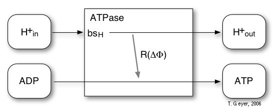 Figure 7: Reactions of the implemented model
of the ATPase.
Figure 7: Reactions of the implemented model
of the ATPase.
For the ATPase an extremenly simplified model with one reaction and one proton binding site bsH is used. The probability for this reaction is, according to experimental observations, modelled by a sigmoidal characteristic depending on the transmembrane potential ∆Φ. For every four H+ taken up via the proton binding site, one ATP is synthesized. The maximal rate, which is reached at ∆Φ = 200 mV, is 100 ATP/s, for which 400 H+/s are required.
The transmembrane potential ∆Φ: the vesicle as a spherical capacitor
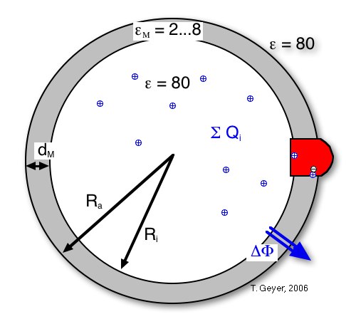
Figure 8: The transmembrane voltage
∆Φ is calculated from the sum of charges inside the vesicle, its
inner radius RM and membrane thickness
dM, and the relative dielectric constant ε
M of the membrane.
This sum of charges includes the protons inside the vesicle, the dipoles from charge separations in the proteins (namely the RCs with oxidized P), and the effective charge on the cytochrome c2 pool, i.e, the difference between the numbers of oxidzed and reduced c2. For the simulation each of these contributions can be included or neglected independently. For convenience an additional charge offset Q0 can be included, which can model, e.g., stably protonated residues.
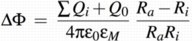
The formula used to calculate ∆Φ is thus:
Implementation of the pools
The pools represent the populations of the different metabolite molecules. Each pool is characterized by the type of molecule it holds, its size, and the number of available molecules of its type.Some pools as, e.g., the pool of protons outside of the vesicle, are so large that the concentration in them is not affected by the action of a small chromatophore vesicle. These pools are then kept fixed during the simulation, i.e., the number of particles inside does not change, even if particles are taken out or put in. Any of the pools can be set fixed to, e.g., look at the behaviour of a single step of the conversion chain under steady state conditions.
According to figure 3, a simulation of the complete vesicle requires a total of eight pools for "real" metabolites, one for the incoming photons and one pools for excitons for each of the LHCs. Consequently, pools for the following metabolites are included in the description:
- photons
- excitons (E) on the bacteriochlorophylls of the LHCs
- protons (H+) outside of the vesicle
- proton (H+) inside of the vesicle
- oxidized quinones (Q)
- reduced quinones (=quinols) (QH2)
- oxidized cytochrome c2 (c2ox)
- reduced cytochrome c2 (c2red)
- ADP outside of the vesicle
- ATP -"-
Not all pools have a three dimensional volume: the quinones, e.g., diffuse in the center of the membrane and it is not clear, how thick this quinone layer is, thus a two dimensional volume is used for the Q and QH2 pools. Analogously, the exciton pools, which store the electronic excitations in the LHCs, are assigned a zero dimensional volume (how many excitons fit into 1 µm3???).
Feeding the vesicles: defining the course of the illumination
By varying the intensity of the light, which is the central metabolite for photosynthesis, many different dynamic scenarios can modelled, ranging from pure steady state working conditions up to the reaction of the photosynthetic chain to very short light pulses.To have maximal freedom in specifying the course of the illumination, only a textbox is provided. Every line specifies a time (the simulation starts at t=0) and a new light intensity in W/m2. Take care that the times are sorted. Via the buttons next to this text box a few predefined illumination profiles can be inserted (and then modified, if desired).
Simulation duration and output interval
The maximal duration for a simulation is limited to 5 million timesteps (e.g., 50 seconds with a timestep of 10 microseconds), which should be sufficient for most scenarios. For comparison, at a timestep of 25 microseconds the simulation of a typical vesicle runs at about real time on our server (P4@2.8GHz).The output interval parameter defines how often the occupation numbers of the pools are reported. The minimal output interval is 0.01 seconds.
References
[1] T. Geyer and V. Helms, "A spatial model of the chromatophore vesicles of Rhodobacter sphaeroides and the position of the cytochrome bc1 complex", Biophys. J. 91 (2006) 921-6[2] T. Geyer and V. Helms, "Reconstruction of a kinetic model of the chromatophore vesicles from Rhodobacter sphaeroides", Biophys. J. 91 (2006) 927-37
[3] T. Geyer, F. Lauck, and V. Helms, "Molecular stochastic simulations of chromatophore vesicles from Rb. sphaeroides", J. Biotech., 129 (2007) 212-228