MutaNET

Automated analysis of genomic Mutations in gene regulatory NETworks

---

Mutations in genomic key elements can influence gene expression and function in various ways, and hence greatly contribute to the phenotype. We developed MutaNET to score the impact of individual mutations on gene regulation and function of a given genome. MutaNET performs statistical analyses of mutations in different genomic regions. The tool also incorporates the mutations in a provided gene regulatory network to estimate their global impact. The integration of a next-generation sequencing pipeline enables calling mutations prior to the analyses. As application example, we used MutaNET to analyze the impact of mutations in antibiotic resistance (AR) genes and their potential effect on AR of bacterial strains.

The following web user guide illustrates the basic usage of MutaNET and how to further process the resulting gene regulatory networks (in .gml format) using Cytoscape visualisation software. The .pdf formatted user guide provides additional information and can be downloaded at Sourceforge or GitHub.

Quickstart

MutaNET comes as Python 3 source code as well as an executable for Windows. Please download MutaNET from Sourceforge. When starting MutaNET for the first time, the file paths for small example data sets for the NGS pipeline, mutation analysis and file converters are already loaded to allow quick testing. Keep in mind that for the NGS pipeline extra programs need to be installed.

Executable (Windows)

To start MutaNET, double–click on the executable MutaNET32.exe or MutaNET64.exe, depending on whether you have a 32–bit or 64–bit Windows installation. If you are not sure, choose the 32–bit executable. Make sure that the executable remains in the same directory as the config.yaml file. Otherwise the user interface will not start.

From Source

Open a command prompt or terminal and execute the following command:

or on Windows depending on your Python installation:

Source_folder_path is the path to the folder containing the source code of MutaNET. This requires Python 3 to be installed. The installation manual explains how to install Python 3, as well as programs required for the NGS pipeline of MutaNET on Windows, Linux and Mac OS X.

Analysis of Staphylococcus aureus antibiotic resistance

Goal

Analysis of the potential impact of mutations on the antibiotic resistance of Staphylococcus aureus with reference strain NCTC 8325.

Data retrieval

There are several data sources available that provide information on gene annotations, protein domains, transcription factors and their binding sites, or antibiotic resistance for multiple bacterial strains. We used the following sources for our analyses. Specific information on file formats and how to use the MutaNET embedded file converter and merger can be found in the .pdf formatted user guide that can be downloaded at Sourceforge.

AureoWiki: Gene information of the reference strain.

UniProt: Protein Domain Analysis.

PATRIC: Antibiotic Resistance database.

RegulonDB: Transcriptional regulation in Escherichia coli K-12.

RegPrecise: Transcription factor (TF) sequences and transcription factor binding site (TFBS) information for the reference strain.

Cytoscape: a program for modeling biological interaction networks in .gml format.

NCBI SRA: Escherichia coli reads were downloaded from the NCBI Sequence Read Archive (SRA), see publication.

Procedure

1. Obtain gene information of the reference strain (e.g. from AureoWiki) as a tab–separated (.tsv) file. Rename relevant columns as specified in Section 3.1.1. of the .pdf user guide (please download at Sourceforge).


2. Generate the mutations file.
   1. Obtain a genome .fasta file of the reference strain. Set the NGS pipeline reference genome file path accordingly.
   2. Obtain NGS reads as paired .fastq files of another strain and place them in a directory. Set the NGS pipeline reads directory accordingly.
   3. Set the NGS pipeline result directory.
   4. Click on NGS pipeline Run.
3. Generate the protein domain file using UniProt.
   1. Open the converter under Tools → UniProt protein domain converter.
   2. Obtain a UniProt protein domain text file of the reference strain as described in Section 4.2.1 of the .pdf user guide (please download at Sourceforge). Set the converter UniProt input file accordingly.
   3. Set the converter result file to an existing .tsv file to override it or create a new one in the file dialog.
   4. Click on Run.
4. Generate the antibiotic resistance file using PATRIC.
   1. Open the converter under Tools → PATRIC antibiotic resistance converter.
   2. Obtain a PATRIC antibiotic resistance file of the reference strain as described in Section 4.3.1 of the .pdf user guide (please download at Sourceforge). Set the converter PATRIC input file accordingly.
   3. Set the converter result file to an existing .tsv file to override it or create a new one in the file dialog.
   4. Click on Run.
5. Search the literature (or any other source) for regulation information and create a regulation .tsv file as specified in Section 3.1.6 of the .pdf user guide (please download at Sourceforge). When analysing Escherichia coli K-12, RegulonDB provides information on transcriptional regulation.


6. Obtain transcription factor (TF) sequences and transcription factor binding site (TFBS) inform- ation for the reference strain (e.g. from RegPrecise). Use that information to create a TFBS .tsv file as specified in Section 3.1.7 of the .pdf user guide (please download at Sourceforge) and a TF multiple sequence alignment file as specified in Section 3.1.8 of the .pdf user guide (please download at Sourceforge).


7. Set the mutation analysis paths.
   1. Set the gene file to the file from step 1.
   2. Set the mutation file to the file in the NGS pipeline result directory from step 2.
   3. Enable Genes of Interest Analysis and set genes of interest file to the file from step 4.
   4. Enable Protein Domain Analysis and set the protein domain file to the file obtained in step 3.
   5. Enabled Coding Region Analysis and set the substitution matrix file to the PAM10 file in the substitution_matrices directory.
   6. Enable Regulation Analysis and set the regulation file to the file created in step 5. 27
   7. Enable Transcription Factor Binding Site Analysis and set the TFBS file and TF MSA file that were created in step 6.
8. Click on mutation analysis Run.

Results

All files listed in Section 3.2. of the .pdf user guide (please download at Sourceforge).

Cytoscape: Gene Regulatory Network (GRN) visualisation

If regulation analysis is enabled, MutaNET will generate a gene regulatory network in .gml format (graph modeling language). This .gml file can be processed by Cytoscape, a program for modeling biological interaction networks. Each node in the .gml file contains information on the (sub–)category of interest it belongs to. Furthermore, the node label contains the number of mutations in the gene: (# non–syn. coding region mutations, # promoter mutations, # TFBS mutations) Each edge contains information on the regulation type: operon (O), activation (A), repression (R), effector (E, can act as activator or repressor) and unknown (?). The following tutorial gives an introduction to how to customise .gml files in Cytoscape.

This is a simple and straightforward explanation on how to open, customise, and finally save a GRN in common formats such as .pdf or .png. For additional information on Cytoscape, please refer to the Cytoscape web page.

1. Download and Installation

Go to Cytoscape and click on download. Navigate to the download folder and execute the installation file you just downloaded and follow the installation instructions. It is very straightforward.

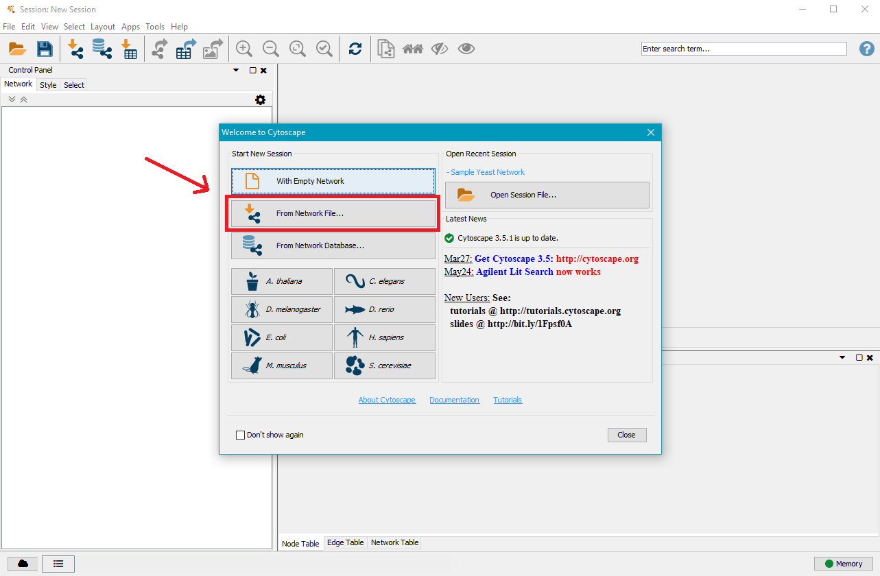
2. Open a .gml file

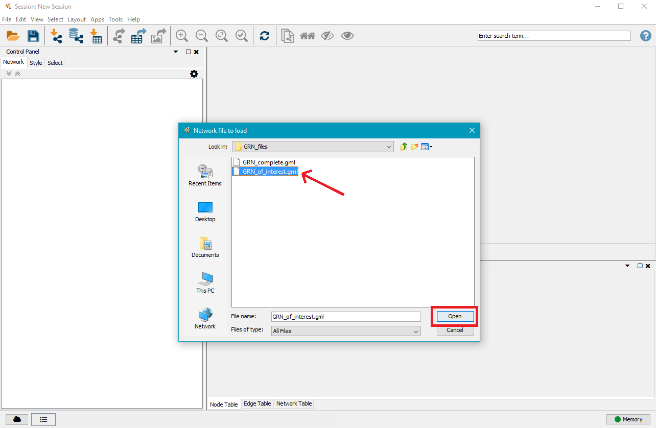
Open Cytoscape and click on From Network File...

Navigate to the mutation analysis results directory and then to the GRN directory contained within, where you will find one or two .gml files. Select the one you want to visualise and click on Open.

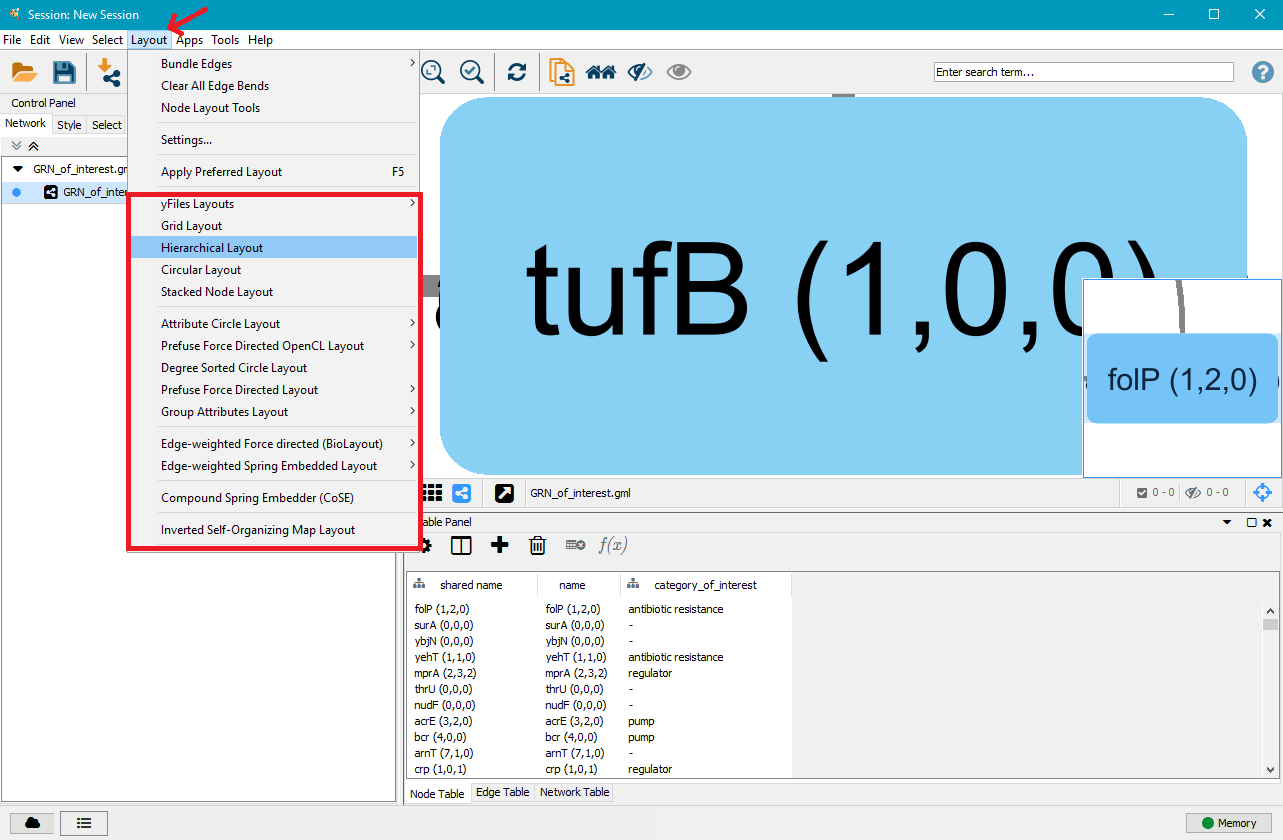
3. Layout your GRN

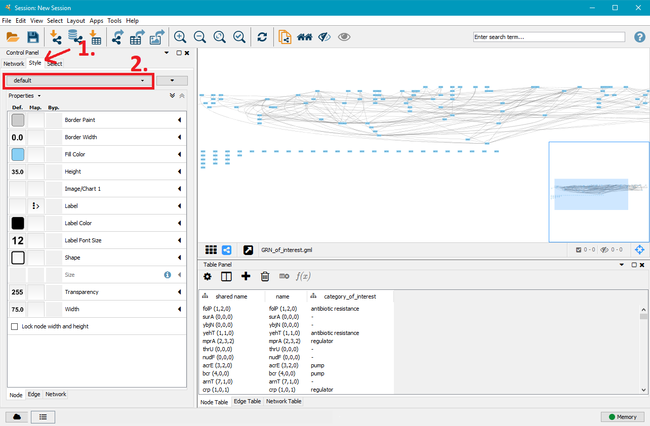
On the right side you will see a large node. That is the current network view. Below is a table with the nodes in the network, with an additional tab for edges. In the top menu bar, click on Layout and select the layout type you wish to apply to the network. In this example we selected Hierarchical Layout, but you can try several layouts and select the one you like the best.

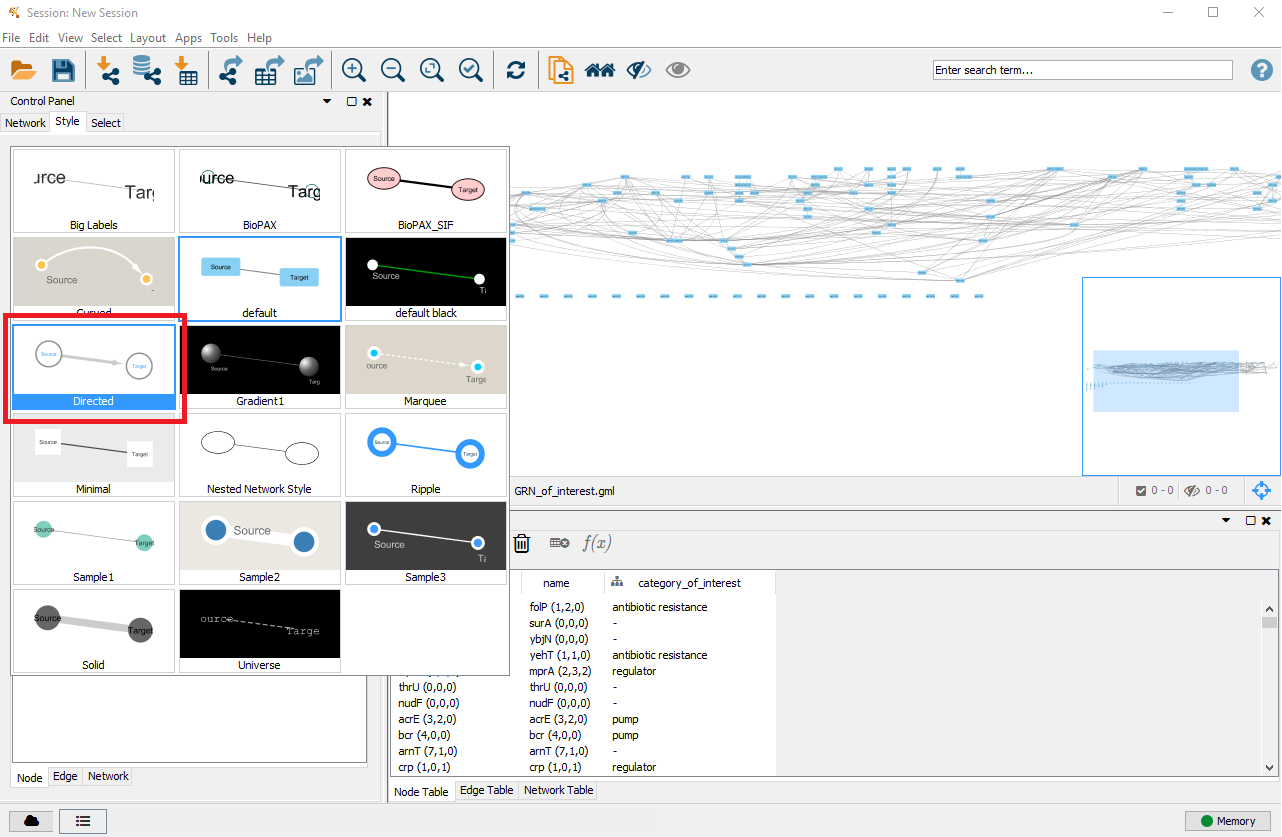
On the right side you can now see that the nodes and edges have been ordered according to the selected layout. You can zoom in and out of the network using the scroll wheel of your mouse, and view different parts of the network by left–clicking and dragging your mouse in the network window. In the top left, click on the Style tab in order to customise the look of your nodes and edges. First, select a network style by clicking on the dropdown menu currently saying default. Select directed.

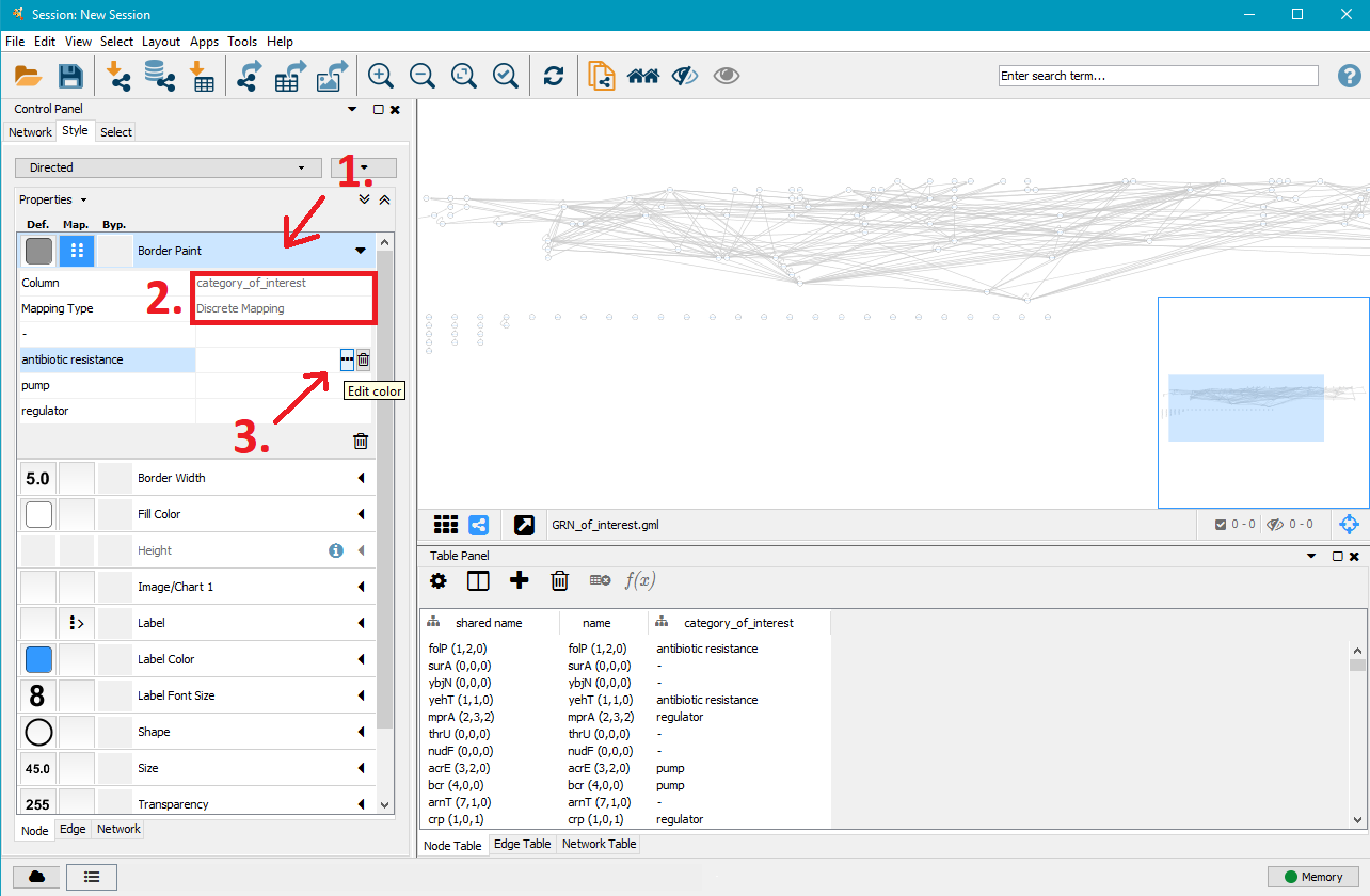
4. Customise node styles

In the left menu you can now customise the colours, shapes, sizes,... of the network nodes. The .gml file gives each node information about the genes of interest (sub–)category it belongs to and Cytoscape allows to apply specific styles to these different node types. In this example we apply different border colours to the nodes depending on their antibiotic resistance. This approach works for all other options given in the style menu.

1. Click on Border Paint to show more options.
2. Click in the field next to Column and select category_of_interest.
3. Click in the field next to Mapping Type and select Discrete Mapping. This will show additional rows listing the (sub–)categories specified in the mutation analysis. In this example, the sub–categories are antibiotic resistance, pump (for multidrug resistance efflux pumps), regulator (for direct multidrug resistance efflux pump regulators) and - (for non–antibiotic resistance genes).
4. Click on the field next to one of the sub–categories, here antibiotic resistance and click on ... to select a border colour of your choice for that node type.

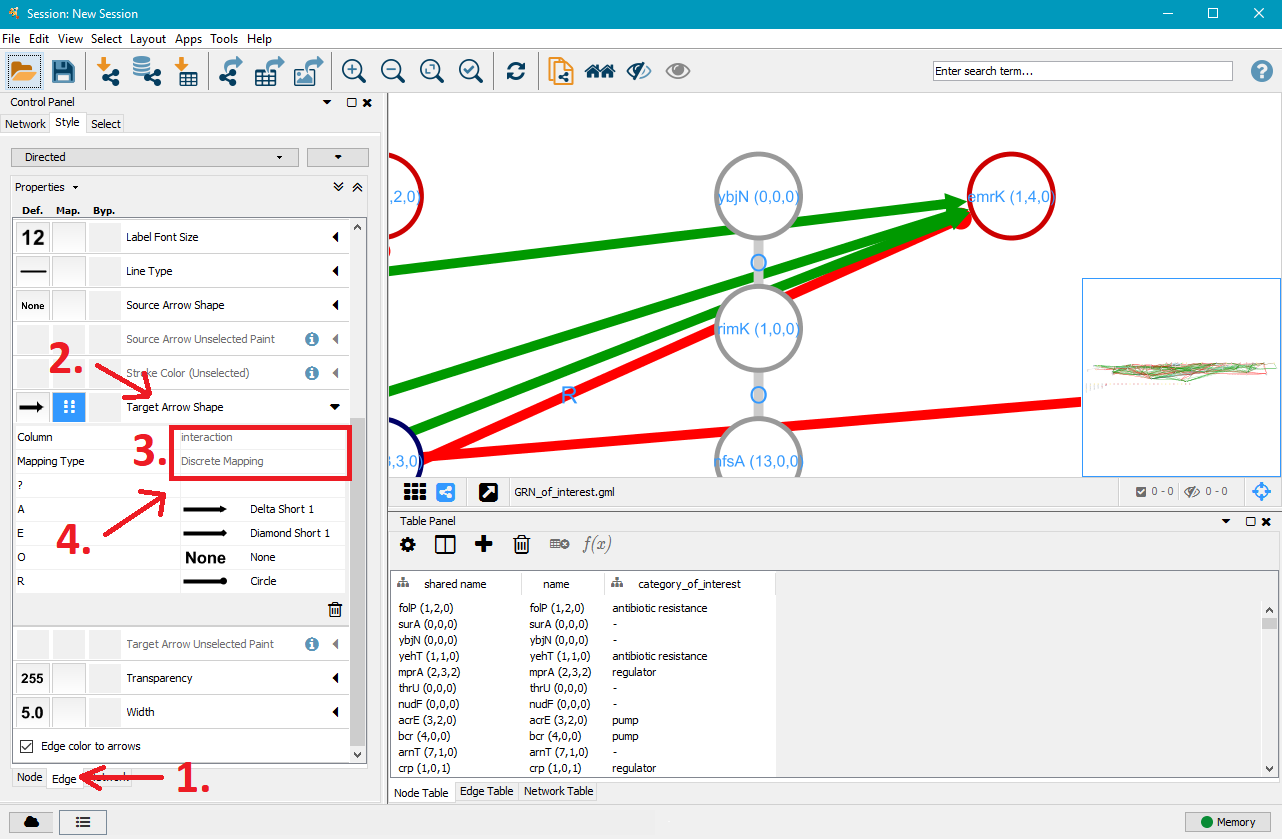
5. Customise edge styles

After you customised the nodes to your liking, click on the Edge tab in the bottom left. This will open a similar menu for edge customisation that works just like the one for nodes. Instead of category_of_interest, select interaction next to Column. This will give you the option to specifically target operon (O), activation (A), repression (R), effector (E, can act as activator or repressor) and unknown (?) interactions.

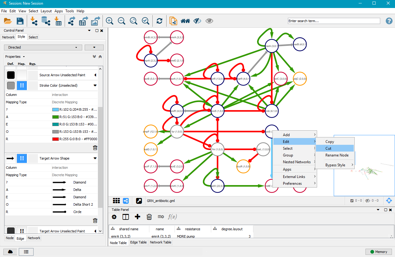
6. Edit/cut nodes and edges

After you customised the edges to your liking, it might be necessary to manually order the network and maybe even remove some unimportant or less important nodes and edges. You can left–click on nodes and drag them to other positions. You can delete nodes and edges by right–clicking on them, selecting Edit and then Cut.

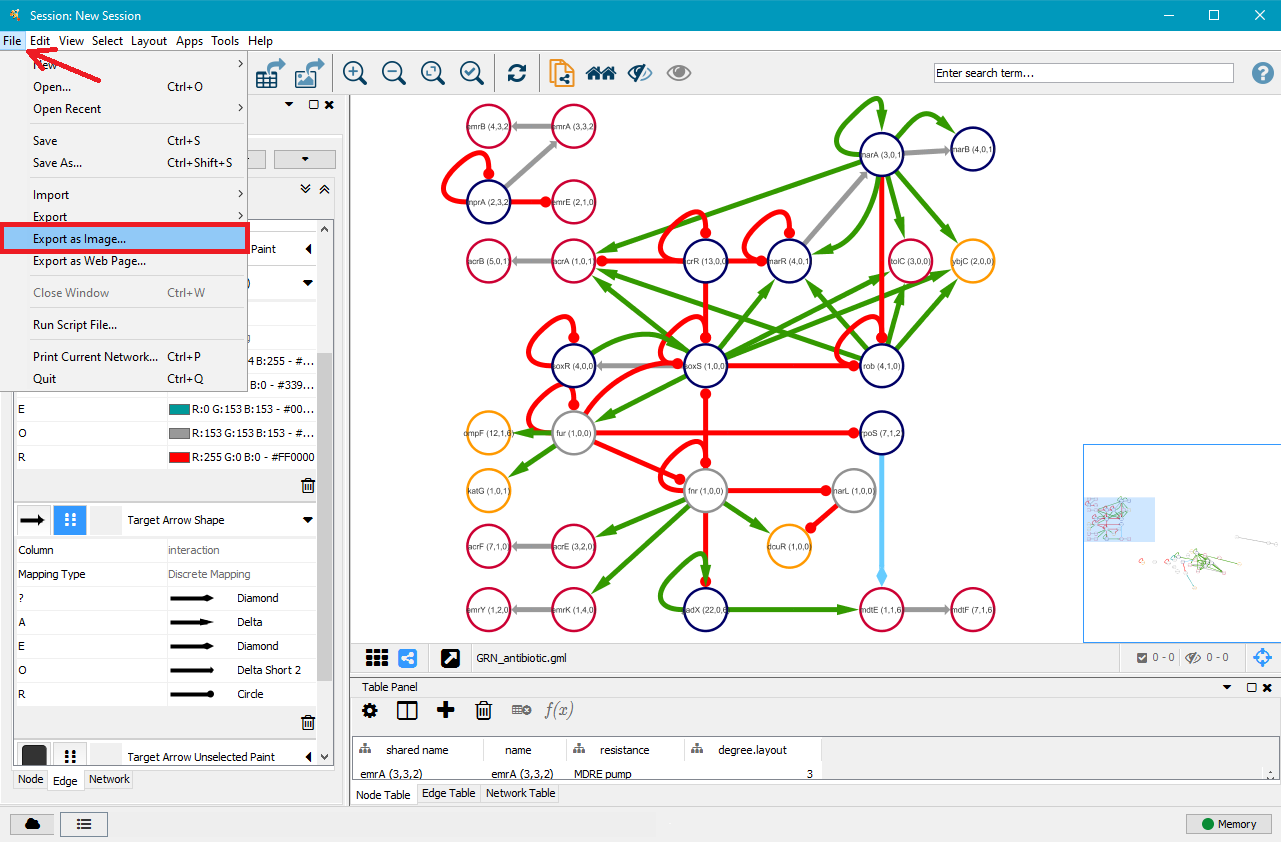
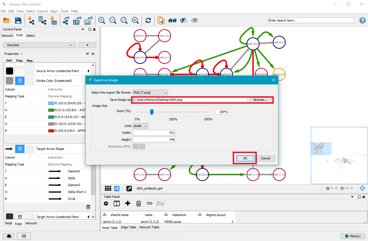
7. Export your GRN as .png, .pdf, .jpeg, .svg or .ps file

Once you are satisfied with your network, you can export it as a .png, .pdf, .jpeg, .svg or .ps file by clicking on File in the top menu and then selecting Export as Image.... Choose the file type and where you want to save it, and then click on OK.